Apache Beam: A Technical Guide to Building Data Processing Pipelines

An In-Depth Look at SDKs, Runners, IOs, and Transformations

Apr 23, 2023

Introduction to Apache Beam

If you’re into data processing and pipelines, you’re in the right place. Apache Beam is an open-source framework that lets you build flexible and scalable data processing pipelines.

At its core, it is all about creating and transforming data. You can use it to read data from various sources (like databases or files), apply transformations to that data (like filtering or aggregating), and write the output to a new destination (like a different database or file format).

But what makes it really special is its flexibility. It allows you to build batch and streaming data processing pipelines with a variety of programming languages (e.g. Java, Python, and Go), and it supports different runners (e.g. Flink, Spark, or GCP Dataflow) that can execute your pipelines in different environments (like on-premises or in the cloud).

Apache Beam is considered a unified programming model because it provides a high-level API that can be used to write data processing pipelines that work seamlessly across different execution engines. This means that you can write your pipeline once and then choose the execution engine that best suits your needs without having to rewrite your code. So, as you see, it’s highly portable, and that is a great quality for a big data tool.

You can look at Apache Beam as a central hub that you can talk with different languages for different data processing purposes (batch or stream) that can run on different engines. That’s why it’s called unified programming model.

Use cases of Apache Beam

So, where can you use this technology? Well, there are lots of possibilities! Here are some common use cases:

Data integration: You can use to integrate data from multiple sources into a single pipeline. For example, you might want to extract data from a database, join it with data from a web service, and then write the results to a file.
ETL (Extract, Transform, Load): It is great for ETL tasks, where you need to transform data from one format to another. For example, you might need to extract data from a legacy system, transform it into a more modern format, and then load it into a new system.
Real-time processing: It also supports windowing, which lets you process data in real-time by grouping it into time-based or event-based windows. For example, you might want to process sensor data from IoT devices in real-time, and take action based on certain patterns or thresholds.

Overview of Apache Beam Architecture

As described earlier, you can look at Apache Beam as an API layer that you can talk to with multiple languages and then run it on various engines to perform batch or stream processing. An interesting fact about Beam is that the name comes from combining Batch and strEAM (BEAM) and shows that the designer had a

Overview of Apache Beam data flow

Also, let’s take a quick look at the data flow and its components. At a high level, it consists of:

Pipeline: This is the main abstraction in Beam. It represents the data processing pipeline that you want to build, and it’s composed of one or more transforms. It’s a graph (specifically direct acyclic graph, i.e. DAG) of all the data and computations of the data processing task.
Transform: This is a data processing operation that takes one or more input PCollections, applies a computation, and produces one or more output PCollections. There are built-in transforms (like “Filter” or “Map”), and you can also create your own custom transforms.
Pcollection: This is a parallel collection of data, it is an immutable object which is the fundamental data structure in Beam. It represents a collection of elements that can be processed in parallel. It doesn’t support grained operation, and random access.

Get Started with Apache Beam

To get started in Python, you’ll first need to install the SDK by running pip install apache-beam in your command prompt or terminal. Once you have the SDK installed, you can create a new Python file to start writing your first Beam pipeline.

Typical pipeline building process looks like this:

Define the pipeline options
Read the input data or create an initial PCollection
Transform the data using using PTransforms such as Map, Filter, GroupByKey, CoGroupByKey, Combine, and Flatten. Each PTransform creates a new PCollection. You can change these transforms together to create the final PCollection.
Run the pipeline using the designated pipeline runner
Then, at the end, write the transformed data to a file or external system

Let’s start with a simple example Beam code to count the number of words in a text file. Imagine you have a following example text file.

word1,word2,word3
hello,world,hello
world,hello,world
foo,bar,foo
bar,baz,foo
baz,foo,bar

Now, you can count the number of words using the following Beam code:

import apache_beam as beam
from apache_beam.options.pipeline_options import PipelineOptions

options = PipelineOptions()

with beam.Pipeline(options=options) as p:
    lines = p | 'ReadFromText' >> beam.io.ReadFromText('input.txt')
    counts = (
        lines
        | 'SplitWords' >> beam.FlatMap(lambda line: line.split(' '))
        | 'CountWords' >> beam.combiners.Count.PerElement()
    )
    counts | 'WriteToText' >> beam.io.WriteToText('output.txt')

I start by importing the apache_beam module and PipelineOptions from the apache_beam.options.pipeline_options module. The module provides options for configuring the Beam pipeline, such as the runner to use and any additional options for the runner. Runner would have its own chapter in this article, so don’t worry about it now.

In this code p refers to the PCollection that runs through the pipeline. Also, in terms of syntaxing, the syntax 'ReadFromText' >> or'SplitWords' >> are used to label the transform with the string 'ReadFromText' or 'SplitWords'. These labels can be useful for debugging and monitoring the pipeline, as they allow you to identify each transform in the pipeline by name.

In this pipeline, I am using beam.io.ReadFromText('input.txt') to read data from a text file, and then applying a FlatMap transform to split each line of text into individual words. I then use beam.combiners.Count.PerElement() to count the number of occurrences of each word in the resulting PCollection. Later in this article, I’m going to break down each of these concepts further.

Finally, I write the word counts to a text file using beam.io.WriteToText('output.txt'). Note that the pipeline is executed when I enter the with block context manager, and the output is written to the output file when I exit the block.

The output would look like this:

('word1', 1)
('word2', 1)
('word3', 1)
('hello', 3)
('world', 3)
('foo', 4)
('bar', 3)
('baz', 2)

Apache Beam SDKs

Now that you know a bit about the basic of Beam, let me explore different SDKs supported by Beam. In this article, I’m going to use Python SDK, but it’s good to know what are the available SDKs and what should be your criteria for choosing one. Apache Beam supports a variety of languages, including Java, Python, Go, and others. Each language has its own SDK, which provides a set of classes and methods for building pipelines.

Overview of different SDKs supported by Apache Beam

Let’s take a quick look at the different SDKs that are available:

Java SDK: This is the original SDK for Apache Beam, and it provides a comprehensive set of classes and methods for building pipelines in Java. The Java SDK is well-documented and well-supported, and it’s a great choice if you’re comfortable with Java.
Python SDK: It is another popular choice for building pipelines in Beam. It is great for prototyping and experimentation. The Python SDK also supports popular libraries like Pandas and TensorFlow.
Go SDK: It is a newer addition to Apache Beam, and it’s still in beta. It provides a lightweight and efficient programming model, and it’s a good choice if you’re already familiar with Go.

Comparison between different SDKs

Each SDK has its own strengths and weaknesses, so it’s important to choose the one that’s best suited to your needs. Here are some factors to consider when choosing an SDK:

Language familiarity: If you’re already comfortable with a particular language, it’s often best to stick with that language’s SDK.
Performance: Some SDKs may be more performant than others, depending on the use case. For example, the Java SDK is generally faster than the Python SDK, but the Python SDK may be easier to work with for small to medium-sized data sets.
Library support: If you’re planning to use third-party libraries like TensorFlow or PyTorch, it’s important to choose an SDK that has good library support. The Python SDK is generally the best choice for library support, but other SDKs may also have good support depending on the library.

Apache Beam runners

After covering SDKs, also it is important to learn about runners. That is where the power of Apache Beam come from. The fact that you can run it on other technologies make it extremely powerful and useful. A runner is basically the engine that executes your pipeline. Apache Beam supports a variety of runners (e.g. Flink, Spark, and GCP Dataflow).

Let’s take a quick look at the different runners that are available:

Apache Flink: It is a popular open-source stream processing framework that can be used as a runner for Apache Beam. Flink provides strong support for stream processing and has good performance for batch processing as well.
Apache Spark: It is popular framework for distributed batch processing. It’s is well-suited for large-scale data processing and provides a unified engine for batch processing, stream processing, and machine learning.
Google Cloud Dataflow: It is a fully-managed service for executing Apache Beam pipelines on the Google Cloud Platform. It is easy to use and provides a scalable and reliable environment for running pipelines. If you are already in GCP ecosystem, it’s a no brainer to use Dataflow.

Each runner obviously has its own strengths and weaknesses, so it’s important to choose the one that’s best suited to your needs. Here are some factors to consider when choosing a runner:

Performance: Some runners may be more performant than others, depending on the use case. For example, Flink is generally faster than Spark for stream processing, while Spark may be faster for batch processing. Obviously, there are more community support for steam processing with Flink and batch processing with Spark.
Ease of use: Some runners may be easier to use than others, depending on your level of experience with the framework. For example, Dataflow is very easy to use, while Apache Flink may have a steeper learning curve. However, if you are on AWS, it might not make sense to use a service from another cloud provider as it doubles your maintenance effort and infrastructure support.
Scalability: Some runners may be more scalable than others, depending on the size of your data and the requirements of your use case. For example, Dataflow is highly scalable and can handle very large data sets, but for other runners, you should pay attention to the implementation and configuration.

Examples of using different runners

Let’s take a look at some examples of using different runners. Obviously runners are configured separately and available to the server. Here’s a simple pipeline that reads from a text file, applies a filter to remove any lines that contain the word “spam”, and writes the results to a new text file:

import apache_beam as beam

# Create the pipeline using the Python SDK and the Dataflow runner.
with beam.Pipeline(runner='DataflowRunner') as p:
    # Read from a text file.
    lines = p | beam.io.ReadFromText('gs://my-bucket/input.txt')

    # Filter out any lines that contain the word "spam".
    filtered_lines = lines | beam.Filter(lambda x: 'spam' not in x)

    # Write the results to a text file.
    filtered_lines | beam.io.WriteToText('gs://my-bucket/output.txt')

And here’s the equivalent pipeline using the Apache Flink runner:

import apache_beam as beam

# Create the pipeline using the Python SDK and the Flink runner.
with beam.Pipeline(runner='FlinkRunner') as p:
    # Read from a text file.
    lines = p | beam.io.ReadFromText('/path/to/input.txt')

    # Filter out any lines that contain the word "spam".
    filtered_lines = lines | beam.Filter(lambda x: 'spam' not in x)

    # Write the results to a text file.
    filtered_lines | beam.io.WriteToText('/path/to/output.txt')

Both examples use Python SDK and the code for the pipeline is largely the same; however, behind the scene, these operations translate differently to interact with their respective runners.

Apache Beam Transformations

Ok. Now that we learned the basic and also SDKs and runners, let’s get deeper into Beam and what it can do. Obviously, in the get started section, I only touched the basics, let’s see what else Beam can offer as a data processing tool. Apache Beam provides a powerful set of transformations, known as PTransforms, that allow you to process data in a variety of ways. In this section, I am planning to cover these PTransforms with example codes of how to use built-in PTransforms, and also show you how to write your own custom PTransforms.

Explanation of PTransforms

It is a fundamental building block in Beam that represents a data processing operation. They take one or more input PCollections and produce one or more output PCollections. PTransforms can be chained together to form complex data processing pipelines.

Beam provides a wide variety of built-in PTransforms that you can use to process data in various ways. These include transforms for reading and writing data, filtering and aggregating data, joining and grouping data, and much more.

Core transforms

The core transforms are a set of built-in transforms that come with the Beam SDK. These transforms provide a set of basic building blocks that can be used to perform common data processing operations.

Some examples of core transforms include:

Map: applies a given function to each element in a PCollection and returns a new PCollection with the transformed elements. There are also a variation of this transform like MapTuple, MapElements, MapKeys, MapValues, and FlatMap. This transform works great with lambda functions, although you can pass any user-defined function.
FlatMap: It’s a 1-to-many transformation. It applies a user-defined function to each input element and outputs zero or more output elements for each input element. For example, you can split a row by a delimiter and flatten it into multiple rows.
Filter: returns a new PCollection containing only the elements that meet a specified condition.
GroupByKey: groups the elements of a PCollection by key and returns a new PCollection where each element is a key-value pair representing a unique key and a list of values associated with that key.
Combine: aggregates the elements of a PCollection and returns a new PCollection with a single output value.
Flatten: merges multiple PCollections into a single PCollection.
Window: divides a PCollection into fixed-size or sliding windows of data, based on a specified time interval or number of elements.
ParDo: The ParDo transform applies a user-defined function to each element in a PCollection, and the output is another PCollection. Later, I’m going to provide more examples of this transform with user-defined logic.

Examples of using built-in PTransforms

Let’s take a look at some examples of using built-in PTransforms. Here’s an example of using the GroupByKey transform to group data by a key:

import apache_beam as beam

with beam.Pipeline() as p:
    # Read from a text file.
    lines = p | beam.io.ReadFromText('/path/to/input.txt')
    # Split the lines into words.
    words = lines | beam.FlatMap(lambda x: x.split())
    # Convert the words to a key-value pair.
    word_counts = words | beam.Map(lambda x: (x, 1))
    # Group the word counts by key.
    grouped_counts = word_counts | beam.GroupByKey()
    # Count the occurrences of each word.
    counts = grouped_counts | beam.Map(lambda x: (x[0], sum(x[1])))
    # Write the results to a text file.
    counts | beam.io.WriteToText('/path/to/output.txt')

In this example, I am reading from a text file, splitting the lines into words, converting the words to a key-value pair, grouping the word counts by key using the GroupByKey transform, counting the occurrences of each word, and writing the results to a new text file. It’s very similar to the example provided in the basics section; however, it uses GroupByKey transform to achieve the same result.

Apache Beam provides many built-in PTransforms, and I try to list and categorize them here. I try my best to use them in the examples I provide in this article to demonstrate how to use them:

Input and Output:

apache_beam.io.ReadFromAvro
apache_beam.io.ReadFromBigQuery
apache_beam.io.ReadFromText
apache_beam.io.ReadFromTFRecord
apache_beam.io.WriteToAvro
apache_beam.io.WriteToBigQuery
apache_beam.io.WriteToText
apache_beam.io.WriteToTFRecord

Basic PTransforms:

apache_beam.transforms.Flatten
apache_beam.transforms.Create
apache_beam.transforms.ParDo
apache_beam.transforms.Filter
apache_beam.transforms.Map
apache_beam.transforms.FlatMap

Aggregator:

apache_beam.combiners.Count
apache_beam.combiners.Mean
apache_beam.combiners.Min
apache_beam.combiners.Max
apache_beam.combiners.Top
apache_beam.combiners.Sample

Key-Value PTransforms:

apache_beam.transforms.GroupByKey
apache_beam.transforms.CoGroupByKey

Windowing:

apache_beam.transforms.WindowInto

Additional:

apache_beam.transforms.Distinct
apache_beam.transforms.Partition
apache_beam.transforms.Reshuffle

Writing custom PTransforms

In addition to using built-in PTransforms, you can also write your own custom ones to process data in a specific way. Writing a custom PTransform involves defining a new class that inherits from the PTransform class (i.e. beam.PTransform) and overrides the expand method.

Here’s an example of how to write a custom PTransform that removes any duplicate values from a PCollection:

import apache_beam as beam

class DedupValues(beam.PTransform):
    def expand(self, pcoll):
        return (
            pcoll
            | beam.Map(lambda x: (x, None))
            | beam.GroupByKey()
            | beam.Keys())

In this example, I define a new class called DedupValues that inherits from the PTransform class. The expand method takes a PCollection as input and returns a new PCollection that has had duplicates removed.

To remove duplicates, I first map each value in the input PCollection to a key-value pair, where the value is set to None. I then group the key-value pairs by key using the GroupByKey transform, and extract the keys to create a new PCollection that contains only unique values.

Once you’ve defined a custom PTransform, you can use it in your data processing pipeline just like any other built-in PTransform.

Apache Beam IOs

Beam provides a variety of I/O connectors for reading and writing data to different data sources. These connectors are designed to be efficient, scalable, and easy to use, and they can be used with different runners and SDKs.

Let’s take a quick look at some of the different I/O connectors that Apache Beam supports:

TextIO: This is used for reading and writing text files. It supports reading and writing files from both local and remote file systems, and it provides a variety of configuration options for customizing the behavior of the connector.
AvroIO: This is used for read/write in/to Avro-formatted data.
BigQueryIO: This is used for I/O to Google BigQuery.
PubSubIO: This is used for reading and writing data to GCP Pub/Sub.
JdbcIO: This connector is for reading and writing data to JDBC databases.

Examples of using different IOs

Let’s take a look at some examples of using different I/O connectors in Beam. Here’s an example of how to read from Google BigQuery and write to a new text file using the BigQueryIO and TextIO connectors:

import apache_beam as beam

with beam.Pipeline() as p:
    # Read from a BigQuery table.
    rows = p | beam.io.ReadFromBigQuery(table='my-project:my-dataset.my-table')
    # Apply a transform to extract the "name" field from each row.
    names = rows | beam.Map(lambda row: row['name'])
    # Write the results to a new text file.
    names | beam.io.WriteToText('/path/to/output.txt')

As you can see, the code for reading and writing data is relatively simple, and the I/O connectors handle the heavy lifting of data processing.

Writing custom IOs

In addition to the built-in I/O connectors, you can also write your own custom I/O connectors to work with data sources that aren’t natively supported. To write a custom I/O connector, you’ll need to define a new class that extends one of the existing I/O connectors, such as FileBasedSource or BoundedSource. You’ll also need to implement methods for reading and writing data to your data source.

Here’s an example of how to write a custom I/O connector for reading and writing data to a MongoDB database:

import apache_beam as beam
import pymongo

class MongoSource(beam.io.iobase.BoundedSource):
    def __init__(self, connection_uri, database, collection):
        self.connection_uri = connection_uri
        self.database = database
        self.collection = collection
    def estimate_size(self):
        client = pymongo.MongoClient(self.connection_uri)
        collection = client[self.database][self.collection]
        return collection.count_documents({})
    def get_range_tracker(self, start_position, stop_position):
        return beam.io.iobase.RangeTracker(start_position, stop_position)
    def read(self, range_tracker):
        client = pymongo.MongoClient(self.connection_uri)
        collection = client[self.database][self.collection]
        cursor = collection.find()
        for document in cursor:
            yield document
class MongoSink(beam.io.iobase.FileBasedSink):
    def __init__(self, connection_uri, database, collection):
        self.connection_uri = connection_uri
        self.database = database
        self.collection = collection
    def open(self, temp_path):
        return pymongo.MongoClient(self.connection_uri)[self.database][self.collection]
    def write_record(self, record, file_handle):
        file_handle.insert_one(record)

This custom I/O connector defines two classes: MongoSource for reading data from a MongoDB database, and MongoSink for writing data to a MongoDB database. These classes extend the BoundedSource and FileBasedSink classes, respectively, and implement the necessary methods for reading and writing data.

Apache Beam Windowing

Apache Beam supports windowing as a way to group data into logical chunks for more efficient processing. Windowing is especially useful when working with streaming data, as it allows you to group data into fixed time intervals or other logical groups. Basically, you can think of windowing as a tool can make Apache Beam a streaming system that is able to handle batch processing as a special case of streaming.

Explanation of windowing

A window is a finite, bounded subset of a PCollection that is defined based on a certain criterion, such as a fixed time interval or a number of elements. Windowing allows you to perform computations on subsets of data, rather than processing all data at once, which can be more efficient and scalable.

When using windowing, data elements are assigned to one or more windows based on the specified criterion. Each window has a start time and an end time, which are used to determine which elements belong to the window. You can perform computations on the elements within each window, and the results are emitted at the end of the window.

Types of windows

There are several types of windows, each of which is suited to different use cases. Here are some of the most common types of windows:

Fixed windows: They divide the data into non-overlapping windows of a fixed duration. For example, you could divide data into 1-minute windows or 1-hour windows. Imagine you have a continuous stream of data, like real-time user clicks, fixed window can be a great fit for analysis of such data.
Sliding windows: They divide the data into overlapping windows of a fixed duration. For example, you could divide data into 5-minute windows that slide by 1 minute.
Session windows: They group data together based on gaps of inactivity between elements. For example, you could group data together that occurs within a certain time period of inactivity. For example, you can define that each user session starts when a user starts clicking in your website and then you close that session when there is a period of 30 minutes inactivity.
Global windows: They treat all data elements as belonging to a single, unbounded window. This is useful for cases where you want to process all data together, such as for a running total.

An illustration of three window types: fixed, sliding, and session.

Example code for windows

Let’s take a look at some examples of using windows in Apache Beam. Here’s an example of how to use a fixed window to count the occurrences of words in a PCollection of text lines:

import apache_beam as beam

with beam.Pipeline() as p:
    # Read from a text file.
    lines = p | beam.io.ReadFromText('/path/to/input.txt')
    # Apply a fixed window of 1 minute.
    windowed_lines = (
        lines
        | beam.WindowInto(beam.window.FixedWindows(60))
        | beam.Map(lambda line: (line, 1))
        | beam.CombinePerKey(sum))

    # Write the results to a new text file.
    windowed_lines | beam.io.WriteToText('/path/to/output.txt')

In this example, I am reading from a text file, applying a fixed window of 1 minute to group the data into minute-long chunks, counting the occurrences of each word in each window, and writing the results to a new text file.

Here’s another example of using a session window to group data based on inactivity:

import apache_beam as beam

with beam.Pipeline() as p:
    # Read from a Pub/Sub topic.
    lines = p | beam.io.ReadFromPubSub(subscription='my-subscription')
    # Apply a session window of 10 seconds.
    windowed_lines = (
        lines
        | beam.WindowInto(beam.window.Sessions(10))
        | beam.Map(lambda line: (line, 1))
        | beam.CombinePerKey(sum))
    # Write the results to a new Pub/Sub topic.
    windowed_lines | beam.io.WriteToPubSub(topic='my-output-topic')

In this example, I am reading from a Pub/Sub subscription, applying a session window of 10 seconds to group the data based on inactivity, counting the occurrences of each data element within each session, and writing the results to a new Pub/Sub topic.

By using windowing, you can efficiently process large amounts of data by breaking it down into smaller, more manageable chunks. This can help you optimize your pipeline’s performance and ensure that it can handle data of any size.

Apache Beam Triggering

Now that we learned about windowing, let’s talk about triggering. Windowing a way for our pipeline to batch the streaming data based on the event timestamp. However, we may not want to process the data right away, or maybe we have some other criteria for when to start processing. So, as you see, processing time is not necessarily equal to event time. That is when triggering comes into the picture. It is a powerful feature that allows you to control how and when your data is processed in a streaming pipeline.

By default, Beam triggers once per window, processing all of the data within that window at once. However, sometimes you may want to process data as it comes in, or you may want to control how often your pipeline processes data within a window.

Beam provides several built-in triggers, including the default trigger mentioned above, as well as triggers for early or late data, processing time-based triggers, and more. You can also create custom triggers to meet your specific processing needs.

Triggers can be set at the pipeline level, the transform level, or even on a per-key basis. They can be combined with other pipeline features, such as windowing and watermarking, to give you even more control over how your data is processed.

One thing to keep in mind is that triggering can have a significant impact on the performance of your pipeline. For example, a trigger that fires frequently may result in higher throughput but may also increase latency. It’s important to consider your use case carefully and choose the trigger that is best suited to your needs.

Let’s see triggers in action. Below code reads a stream of words from Pub/Sub and outputs the top 3 most frequently occurring words every 5 seconds using a FixedWindows trigger:

import apache_beam as beam
from apache_beam import window
from apache_beam.options.pipeline_options import PipelineOptions
from apache_beam.transforms.trigger import AfterProcessingTime
from apache_beam.transforms.trigger import AccumulationMode

class ExtractWords(beam.DoFn):
    def process(self, element):
        for word in element.split():
            yield word

class CountWords(beam.PTransform):
    def expand(self, pcoll):
        return (pcoll
                | 'ExtractWords' >> beam.ParDo(ExtractWords())
                | 'CountWords' >> beam.combiners.Count.PerElement()
                )

options = PipelineOptions()

with beam.Pipeline(options=options) as p:
    (p | 'ReadFromPubSub' >> beam.io.gcp.pubsub.ReadFromPubSub(subscription='projects/<PROJECT_ID>/subscriptions/<SUBSCRIPTION_ID>')
       | 'WindowIntoFixedWindows' >> beam.WindowInto(window.FixedWindows(5), trigger=AfterProcessingTime(2), accumulation_mode=AccumulationMode.DISCARDING)
       | 'CountWords' >> CountWords()
       | 'TopN' >> beam.transforms.combiners.Top.Of(3, key=lambda x: x[1])
       | 'FormatOutput' >> beam.Map(lambda x: f"{x[0]}: {x[1]}")
       | 'WriteToLog' >> beam.io.WriteToText('output')
    )

If the syntax is too heavy, don’t worry, you can check the next section to see more example codes and then return to this example that showcases triggers in Beam.

In this example, the WindowIntoFixedWindows transform is used to partition the incoming stream of words into 5-second fixed windows. The AfterProcessingTime(2) trigger is specified to emit results every 2 seconds. The AccumulationMode.DISCARDING parameter ensures that the trigger discards all data that is not currently in a window.

The output of this pipeline is the top 3 most frequently occurring words in each 5-second window, written to a text file.

Apache Beam in Action

Ok. I personally the best way to learn a technology is to see it in action. Let’s explore different example codes and see how it performs data processing.

Let’s do some processing on the following data

Date,Product,Price,Quantity
2022-01-01,Product A,10.99,5
2022-01-01,Product B,5.99,10
2022-01-02,Product A,9.99,7
2022-01-02,Product C,19.99,3
2022-01-03,Product B,5.99,12
2022-01-03,Product D,29.99,2
2022-01-04,Product A,10.99,4
2022-01-04,Product C,19.99,6
2022-01-05,Product B,5.99,8
2022-01-05,Product D,29.99,3
2022-01-06,Product A,10.99,3
2022-01-06,Product C,19.99,4
2022-01-07,Product B,5.99,15
2022-01-07,Product D,29.99,5
2022-01-08,Product A,10.99,6
2022-01-08,Product C,19.99,8
2022-01-09,Product B,5.99,18
2022-01-09,Product D,29.99,7
2022-01-10,Product A,10.99,9
2022-01-10,Product C,19.99,10

Let’s add it to a csv file sales.csv. Now let’s compute the total sales for each product.

import apache_beam as beam
from apache_beam.options.pipeline_options import PipelineOptions

options = PipelineOptions()

with beam.Pipeline(options=options) as p:
    sales = (
        p
        | 'ReadSalesData' >> beam.io.ReadFromText('sales.csv', skip_header_lines=1)
        | 'ParseSalesData' >> beam.Map(lambda line: line.split(','))
        | 'FilterSalesData' >> beam.Filter(lambda fields: len(fields) == 4)
        | 'ParsePriceQuantity' >> beam.Map(lambda fields: (float(fields[2]), int(fields[3])))
        | 'ComputeSalesByProduct' >> beam.CombinePerKey(sum)
        | 'FormatSalesData' >> beam.Map(lambda item: f"{item[0]}: {item[1]} sales")
        | 'WriteSalesData' >> beam.io.WriteToText('sales_output.txt')
    )

This is the breakdown of what happens in this code:

I import the apache_beam module and PipelineOptions from the apache_beam.options.pipeline_options module.
I create a new instance of PipelineOptions with default options.
I create a new pipeline using the beam.Pipeline constructor, passing in the PipelineOptions instance.
I use the pipeline object p to read the sales data from a CSV file using beam.io.ReadFromText('sales.csv', skip_header_lines=1). I skip the first line of the file, which contains the header row.
I apply a Map transform to each line of text in the sales data to split it into fields using lambda line: line.split(',').
I apply a Filter transform to remove any lines with an incorrect number of fields using lambda fields: len(fields) == 4.
I apply a Map transform to extract the price and quantity fields from each sales record and convert them to floats and integers using lambda fields: (float(fields[2]), int(fields[3])).
I apply a CombinePerKey transform to compute the total sales for each product using sum.
I apply a Map transform to format the sales data as strings using lambda item: f"{item[0]}: {item[1]} sales".
Finally, I use beam.io.WriteToText('sales_output.txt') to write the formatted sales data to a text file named sales_output.txt.

The result is:

10.99: 27 sales
5.99: 63 sales
9.99: 7 sales
19.99: 31 sales
29.99: 17 sales

Now, let’s make it a bit more advanced and add more processing to the mix. Here, I try to group the sales data by date and product, and compute the total sales and average price per product per day.

import apache_beam as beam

# Define a function to parse the input lines and extract the fields
def parse_input(line):
    date, product, price, quantity = line.split(',')
    return (date, product), (float(price), int(quantity))

# Define a function to format the output
def format_output(key, value):
    (date, product) = key
    total_sales = value[0]
    avg_price = value[0] / value[1]
    return f"{date},{product},{total_sales:.2f},{avg_price:.2f}"

# Define the pipeline
with beam.Pipeline() as pipeline:
    # Read the input file
    lines = pipeline | beam.io.ReadFromText('sales.csv')

    # Parse the input lines and group by key
    grouped = lines | beam.Map(parse_input) | beam.GroupByKey()

    # Compute the total sales and average price per product per day
    sales = grouped | beam.Map(lambda x: (x[0], (sum(p[0]*p[1] for p in x[1]), sum(p[1] for p in x[1]))))
    results = sales | beam.Map(lambda x: format_output(x[0], x[1]))

    # Write the output to a file
    results | beam.io.WriteToText('output.txt')

First, I import the apache_beam library and then I define two helper functions to parse the input lines and format the output.

I then define the pipeline using the with beam.Pipeline() as pipeline: statement, and read the input data from a file named sales.csv using the beam.io.ReadFromText method.

Then I apply a series of transformations to the input data to compute the total sales and average price per product per day. First, I use the beam.Map method to apply the parse_input function to each input line, and group the data by key (date, product) using the beam.GroupByKey method.

Next, I use another beam.Map method to compute the total sales and quantity for each product per day. I do this by using a lambda function that takes each (key, value) pair and returns a tuple of the same key and a value that is a tuple of the total sales and total quantity. Next, I compute the total sales by multiplying the price and quantity for each sale, and summing them up using a generator expression. I also sum up the quantities using another generator expression.

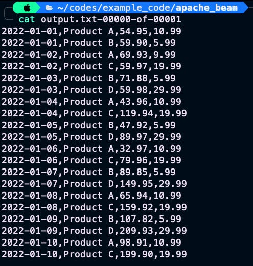
Finally, I use another beam.Map method to apply the format_output function to each (key, value) pair and format the output into a string. I then write the output to a file named output.txt using the beam.io.WriteToText method. The end result would look like this:

Now, let’s see how we can use user-defined functions. Assume below is our input data and we want to count words in the data and filter only words that occurs more than 10 times.

The quick brown fox jumps over the lazy dog
The quick brown fox jumps over the lazy dog
The quick brown fox jumps over the lazy dog
The quick brown fox jumps over the lazy dog
The quick brown fox jumps over the lazy dog
The quick brown fox jumps over the lazy dog
The quick brown fox jumps over the lazy dog
The quick brown fox jumps over the lazy dog
The quick brown fox jumps over the lazy dog
The quick brown fox jumps over the lazy dog
The quick brown fox jumps over the lazy dog
apple banana orange
apple apple orange orange orange
orange orange orange orange orange

Now see the code:

import apache_beam as beam
from apache_beam.io import ReadFromText
from apache_beam.io import WriteToText
from apache_beam.options.pipeline_options import PipelineOptions

# Define the pipeline options
options = PipelineOptions()

# Define a class to filter and count words
class FilterAndCountWords(beam.DoFn):
    def process(self, element):
        word, count = element
        if count > 10:
            yield word, count

# Define the pipeline
with beam.Pipeline(options=options) as pipeline:
    # Read input file
    lines = pipeline | 'Read' >> ReadFromText('input.txt')

    # Split the lines into words
    words = lines | 'Split' >> beam.FlatMap(lambda line: line.split())

    # Count the occurrence of each word
    counts = words | 'Count' >> beam.combiners.Count.PerElement()

    # Filter and count words with count > 10
    filtered_counts = counts | 'Filter' >> beam.ParDo(FilterAndCountWords())

    # Write the output to a file
    filtered_counts | 'Write' >> WriteToText('output.txt')

First, I define a class called FilterAndCountWords that extends the beam.DoFn class. This class is used as the implementation for the beam.ParDo transform that filters and counts the words.

The beam.DoFn class is a base class for user-defined functions in Beam that can be used in beam.ParDo transforms. It provides a process method that takes an input element and produces zero or more output elements. I define a process method in the FilterAndCountWords class to filter and count the words.

In the process method, I take an input element, which is a tuple of a word and its count. I extract the word and count values from the input element, and check if the count is greater than 10. If the count is greater than 10, I yield the input element as output. Otherwise, I don't yield anything, effectively filtering out the word.

I use the beam.ParDo transform to apply the FilterAndCountWords class to the counts PCollection. beam.ParDo takes the user-defined function class as an argument, and creates a new PCollection with the output elements produced by the function.

Using beam.ParDo allows to implement more complex data processing logic than I could with beam.FlatMap. I can use the beam.DoFn class to define more complex processing steps that involve multiple input and output elements, and can even maintain state across multiple processing steps if needed.

The result is:

Now as a final example, let’s define a pipeline to read logs from a text file, filter and process them to get insight about the data. Below is log file of different endpoints in our API and the response code and the response time.

2022-04-08T13:23:45.678Z,192.168.1.1,/endpoint1,200,0.123
2022-04-08T13:24:45.678Z,192.168.1.2,/endpoint2,404,0.234
2022-04-08T13:25:45.678Z,192.168.1.3,/endpoint1,200,0.345
2022-04-08T13:26:45.678Z,192.168.1.4,/endpoint3,200,0.456
2022-04-08T13:27:45.678Z,192.168.1.5,/endpoint2,200,0.567
2022-04-08T13:28:45.678Z,192.168.1.6,/endpoint1,200,0.678
2022-04-08T13:29:45.678Z,192.168.1.7,/endpoint2,200,0.789
2022-04-08T13:30:45.678Z,192.168.1.8,/endpoint1,200,0.890
2022-04-08T13:31:45.678Z,192.168.1.9,/endpoint3,404,0.901
2022-04-08T13:32:45.678Z,192.168.1.10,/endpoint1,200,1.012
2022-04-08T13:33:45.678Z,192.168.1.11,/endpoint2,200,1.123
2022-04-08T13:34:45.678Z,192.168.1.12,/endpoint3,200,1.234
2022-04-08T13:35:45.678Z,192.168.1.13,/endpoint1,200,1.345
2022-04-08T13:36:45.678Z,192.168.1.14,/endpoint2,200,1.456
2022-04-08T13:37:45.678Z,192.168.1.15,/endpoint1,200,1.567
2022-04-08T13:38:45.678Z,192.168.1.16,/endpoint2,200,1.678
2022-04-08T13:39:45.678Z,192.168.1.17,/endpoint3,200,1.789
2022-04-08T13:40:45.678Z,192.168.1.18,/endpoint1,200,1.890
2022-04-08T13:41:45.678Z,192.168.1.19,/endpoint2,404,2.012
2022-04-08T13:42:45.678Z,192.168.1.20,/endpoint3,200,2.123

The code to find popular endpoints and average response time of each endpoint.

import apache_beam as beam
from apache_beam.io import ReadFromText
from apache_beam.io import WriteToText
from apache_beam.options.pipeline_options import PipelineOptions

# Define the pipeline options
options = PipelineOptions()

# Define a function to filter and count words
def filter_and_count_words(element):
    word, count = element
    if count > 10:
        yield word, count

# Define a function to parse a log line into a dictionary
def parse_log_line(line):
    fields = line.split(',')
    return {
        'timestamp': fields[0],
        'ip_address': fields[1],
        'endpoint': fields[2],
        'response_code': int(fields[3]),
        'response_time': float(fields[4])
    }

# Define a class to calculate the average response time per endpoint
class CalculateAverageResponseTimePerEndpoint(beam.DoFn):
    def process(self, element):
        endpoint, logs = element
        response_times = [log['response_time'] for log in logs]
        num_responses = len(response_times)
        total_response_time = sum(response_times)
        avg_response_time = total_response_time / num_responses
        yield endpoint, avg_response_time


# Define the pipeline
with beam.Pipeline(options=options) as pipeline:
    # Read input file
    logs = pipeline | 'Read' >> ReadFromText('input.txt')

    # Parse log lines into dictionaries
    parsed_logs = logs | 'Parse' >> beam.Map(parse_log_line)

    # Filter logs with response code 200
    filtered_logs = parsed_logs | 'Filter' >> beam.Filter(lambda log: log['response_code'] == 200)

    # Transform logs into key-value pairs where the keys are endpoints and the values are 1
    endpoint_counts = filtered_logs | 'EndpointCounts' >> beam.Map(lambda log: (log['endpoint'], 1)) | 'CountEndpoints' >> beam.combiners.Count.PerKey()

    # Filter endpoints with count > 1000
    popular_endpoints = endpoint_counts | 'FilterEndpoints' >> beam.Filter(lambda endpoint_count: endpoint_count[1] > 5)

    # Group logs by endpoint and calculate the average response time per endpoint
    grouped_logs = filtered_logs | 'GroupByEndpoint' >> beam.GroupBy(lambda log: log['endpoint'])
    avg_response_times = grouped_logs | 'CalculateAvgResponseTime' >> beam.ParDo(CalculateAverageResponseTimePerEndpoint())

    # Write the output to files
    popular_endpoints | 'WritePopularEndpoints' >> WriteToText('popular_endpoints.txt')
    avg_response_times | 'WriteAvgResponseTimes' >> WriteToText('avg_response_times.txt')

The pipeline starts with defining options for the pipeline using the PipelineOptions class. Then, it defines a function filter_and_count_words that filters and counts words based on a count condition. Next, there is a function parse_log_line that parses each log line into a dictionary with specific fields such as timestamp, IP address, endpoint, response code, and response time.

The pipeline then starts with reading input from a text file input.txt using ReadFromText function and applies the parse_log_line function to each line of the input file using beam.Map. The output of this transformation is then filtered to include only those logs with response code 200 using beam.Filter.

The filtered logs are then transformed into key-value pairs, where the keys are endpoints and the values are 1 using beam.Map. This transformation is then followed by a combiner transformation beam.combiners.Count.PerKey() that counts the number of occurrences of each endpoint in the input logs.

The pipeline then filters out popular endpoints that have count greater than 5 using beam.Filter transformation. Obviously 5 hit is not an indicator of popularity, but here since the sample data is small, I picked 5 as a threshold of popularity. The logs are then grouped by endpoint using beam.GroupBy transformation. Finally, the average response time per endpoint is calculated using a custom CalculateAverageResponseTimePerEndpoint class that implements beam.DoFn interface. This is done by taking the list of logs for each endpoint, calculating the total response time, and then dividing it by the number of responses.

Finally, the output is written to two text files — popular_endpoints.txt and avg_response_times.txt using WriteToText function.

Advanced topics

In addition to the basics of Apache Beam, there are a number of advanced topics that you may want to explore if you’re using the framework for more complex data processing tasks. In this section, I am going to cover three of these topics: fault tolerance, optimization techniques, and monitoring and debugging.

Fault tolerance in Apache Beam

Fault tolerance is a critical aspect of any distributed data processing framework. In Beam, fault tolerance is achieved through a combination of checkpointing and retries.

Checkpointing involves periodically writing intermediate results to persistent storage, which allows the pipeline to recover from failures by restarting from the most recent checkpoint. Retries involve re-executing failed tasks, either on the same or a different worker, until they complete successfully.

Apache Beam provides several configuration options for controlling the level of fault tolerance in your pipeline, including the frequency of checkpointing and the number of retries.

Optimization techniques in Apache Beam

To achieve the best possible performance, it’s important to apply optimization techniques such as fusion, partitioning, and batching.

Fusion involves combining multiple transforms into a single composite transform, which can reduce the overhead of data serialization and deserialization. For example, in the first example of the previous section, multiple transformation were fused together. I just repeat the fused part below for your reference:

with beam.Pipeline(options=options) as p:
    sales = (
        p
        | 'ReadSalesData' >> beam.io.ReadFromText('sales.csv', skip_header_lines=1)
        | 'ParseSalesData' >> beam.Map(lambda line: line.split(','))
        | 'FilterSalesData' >> beam.Filter(lambda fields: len(fields) == 4)
        | 'ParsePriceQuantity' >> beam.Map(lambda fields: (float(fields[2]), int(fields[3])))
        | 'ComputeSalesByProduct' >> beam.CombinePerKey(sum)
        | 'FormatSalesData' >> beam.Map(lambda item: f"{item[0]}: {item[1]} sales")
        | 'WriteSalesData' >> beam.io.WriteToText('sales_output.txt')
    )

Partitioning involves dividing your data into smaller partitions, which can improve parallelism and reduce the amount of memory required to process each partition. Look at the below example:

import apache_beam as beam

# Define the number of partitions
num_partitions = 2

# Define a function to determine the partition of each element
def determine_partition(element, num_partitions):
    if element % num_partitions == 0:
        return 0
    else:
        return 1

# Create a pipeline
with beam.Pipeline() as pipeline:
    # Create a PCollection of numbers
    numbers = pipeline | beam.Create(range(20))

    # Partition the PCollection into two partitions
    partitioned_numbers = numbers | beam.Partition(determine_partition, num_partitions)

    # Write the output of each partition to a separate file
    for i in range(num_partitions):
        partitioned_numbers[i] | f'WritePartition{i}' >> beam.io.WriteToText(f'partition{i}.txt')

Batching involves processing data in batches, rather than individual records, which can reduce the overhead of data serialization and improve the efficiency of I/O operations. Here is an example of putting your data into batches:

import apache_beam as beam

with beam.Pipeline() as pipeline:
    # Create a PCollection of integers
    pcoll = pipeline | beam.Create(range(1,10))

    # Convert the integers into key-value pairs
    key_value_pcoll = pcoll | beam.Map(lambda x: ('key', x))

    # Group the key-value pairs into batches of size 3
    batches = key_value_pcoll | beam.GroupIntoBatches(3)

    # Print the batches
    batches | beam.Map(print)

Apache Beam provides a variety of tools and techniques for optimizing your pipeline, including the ability to manually fuse transforms, apply automatic partitioning, and configure batch size.

Monitoring and debugging pipelines

Finally, it’s important to be able to monitor and debug your Apache Beam pipeline to ensure that it’s running smoothly and efficiently. It provides several tools and techniques for monitoring and debugging your pipeline, including Beam metrics, logging, and visualization tools.

Beam metrics allow you to monitor key performance indicators for your pipeline, such as processing time, memory usage, and throughput. Logging allows you to capture detailed information about your pipeline’s execution, such as error messages and warnings. Visualization tools allow you to visualize the execution plan of your pipeline and identify bottlenecks and performance issues.

By using these monitoring and debugging tools, you can identify and resolve performance issues in your pipeline quickly and efficiently.

Conclusion

In this article, I covered the basics of Apache Beam, including the different SDKs, runners, and best practices for writing data processing pipelines. Apache Beam is a powerful and flexible framework for processing both batch and streaming data, and it can be used with a variety of different data processing engines and platforms, and I tried my best to provide enough example to demonstrate the strength of this technology.

If you’re new to Apache Beam, I recommend starting with the official Apache Beam website, which provides a variety of tutorials, examples, and documentation to help you get started. You can also explore the source code on GitHub to see how the framework works under the hood.

I hope this article has provided you with a solid foundation for understanding Beam and how it can be used to process data at scale. Whether you’re working with small data sets or petabytes of data, it provides a powerful and flexible framework for processing data efficiently and effectively.

If you have any questions or feedback on this article, feel free to leave a comment on this article and I try to be responsive.

References

Apache Beam Explained in 12 Minutes (link)
Apache Beam Python SDK (link)
Apache Beam Documentation (link)
Apache Beam SDKs (link)
Apache Beam Basics (link)
Apache Beam Pipeline construction and runtime (link)
Event-Driven Systems: A Deep Dive into Pub/Sub Architecture (link)
From Hadoop to Spark: An In-Depth Look at Distributed Computing Frameworks (link)
Five must-read books for data engineers (link)
Data Solution Architects: The Future of Data Management (link)
Data Orchestration 101: Understanding the Different Types of Tools and Their Use Cases (link)

I hope you enjoyed reading this 🙂. If you’d like to support me as a writer consider signing up to become a Medium member. It’s just $5 a month and you get unlimited access to Medium 🙏 .
Before leaving this page, I appreciate if you follow me on Medium and Linkedin 👉
Also, if you are a medium writer yourself, you can join my Linkedin group. In that group, I share curated articles about data and technology. You can find it: Linkedin Group. Also, if you like to collaborate, please join me as a group admin.

Level Up Coding

Thanks for being a part of our community! Before you go:

👏 Clap for the story and follow the author 👉
📰 View more content in the Level Up Coding publication
💰 Free coding interview course ⇒ View Course
🔔 Follow us: Twitter | LinkedIn | Newsletter

🚀👉 Join the Level Up talent collective and find an amazing job

Tech Lead Curiosity

Discussion about this post